Merging Structural Variant Calls from Different Callers
As part of the work of the Pancancer variant-calling working group, we needed to merge the results of variant calls from a wide range of different packages to compare their results and select interesting sites for lab validation. This is a more subtle procedure than it sounds, and we could not find any one place where all the necessary information was documented, so we wrote up our process here. Code that implements this part of our analysis pipeline can be found on GitHub.
Simple Variants - SNVs, Indels
The standard format used to output variants is the Variant Call Format. For SNVs and shortish indels (insertions or deletions), this works very well. Each entry in a VCF file contains the location of the variant (the chromosome it occurs on, and the starting position), the relevant excerpt of the reference sequence starting at that position, and the “alternate” sequence – the variant sequence that has been found there instead.
There are other fields that we will come back to; but a VCF file containing an A → G SNV at chromosome 1, position 100, a 3 base-pair deletion at chromosome 2, position 200, and a 5 basepair insertion at chromosome 3, position 300 would look something like this:
#CHROM POS  ID  REF     ALT     ..
1       100 .   A       G
2       200 .   CGTA    C
3       300 .   T       TACGTA
Even this admits some ambiguity; for instance, a deletion of 3 As within a homopolymer run of 10 of them could reasonably be called at any of 8 positions; and more complex substitions can be equally described as one large variant, or as a combination of insertions, deletions, and substitions. To break these ambiguities, there is a well understood normalization process, which requires looking at both the reference genome and the VCF file. It is fairly straightforward, implemented by several tools, and we perform this step (using bcftools norm) upon ingesting the submitted calls from various groups.
Once these sorts of calls are normalized, they are fairly easily merged and compared. We used python for this project, and we used Jared’s code from an earlier pilot for this – using a dictionary of dictionaries, where the first key was a (chromosome,start position) tuple. The value in the first dictionary corresponding to that key was then a dictionary of (reference allele, variant allele), with a value that was a list of callers that had made that call. So querying existance of a variant was just two (at most) dictionary lookups; and registering that a caller made a particular call was two dictionary lookups and a list append, possibly creating dictionaries and lists along the way if this was the first time these entries were seen.
Structural Variants
Performing the same task with structural variants (henceforth SVs) was more complicated for two reasons:
- Location - by nature of how SVs are detected, there is quite often uncertainty in the position of called SVs, making comparison more complicated; and
- Description - there are a large number of ways that callers actually call SVs, and they need to be converted to some common representation for comparison.
Location
Structural variants are generally observed differently than, say, SNVs. An alignment-based method might align a read to a reference, find that the alignment unambigiously implies a mismatch, and so call an SNV, as in the top panel of the figure below; there is no question about the location of the variant. (Obviously, to call the variant with any confidence would require multiple reads, not shown in the figure for clarity.)
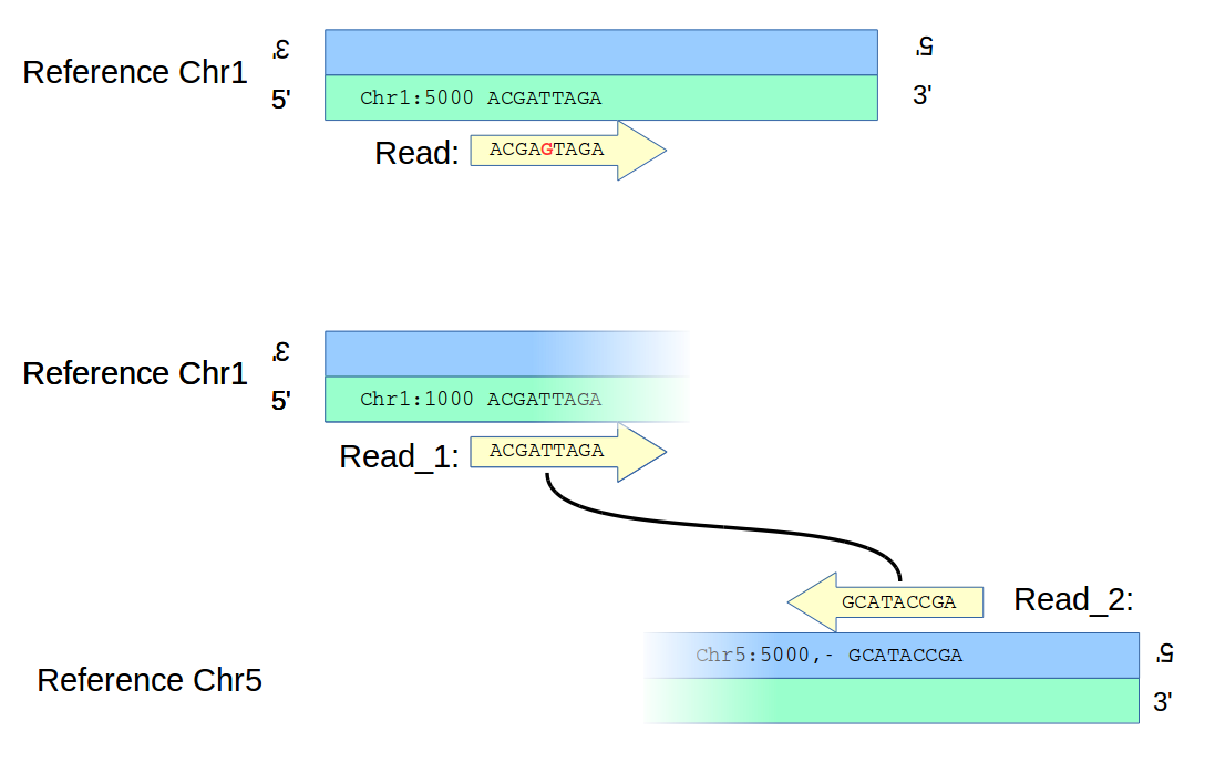
However, a structural variant – say a translocation, as in the bottom panel of the figure – will likely be found differently. In the diagram, paired ends of a read map to two different chromosomes unambigiously, but there is ambiguity as to the location of the two breakpoints on the chromosomes which are now joined to form an new adjacency. Information from other reads will reduce the uncertainties, even to zero; but in the general case one has to handle ambiguity in location when deciding which calls to merge.
Many callers provided confidence intervals on locations of the breakpoints in their calls, which could be used for constraining the merging of calls. However, not all callers did; and there was, naturally enough, significant variation in the confidence intervals, even for a given variant. Thus we took a simpler approach, merging using a fixed window size. Two calls, where each breakpoint of one call was less than the window size away from the corresponding breakpoint of the other call, were merged.
We used a fixed window size of 300bp, of the order of the insert size observed in the libraries; in principle, this is a more agressive merging strategy than using the confidence intervals when available (which were typically much less), but in practice, there were very few pairs of calls where the larger window size would have mattered.
The most efficient way to look up possible matching locations within some window would be to use a spatial data structure such as an interval tree; however, since our window size was relatively modest, and we are constrained to integer positions, I dealt with uncertainty in locations in location lookups by brute-force; I simply search every integer position within the window. For efficiency, and to ensure the closest match is found, the search is by distance (pos+0, pos±1, …). Because dictionary lookup in python is so fast, this approach is “fast enough” for our purposes, in that this is not the rate limiting step for the merging pipeline.
Description
A bigger challenge – not conceptually, but in terms of bookkeeping and corner cases – is simply the diversity of ways in which calls are labelled in VCF files by various callers.
Breakpoint notation (SVTYPE=BND)
The VCF Standard describes two ways of describing SVs in a VCF file, of which there are numerous small variations out in the field. The second, described in somewhat more detail, is breakend notation (usually labelled with an SVTYPE=BND entry in the INFO field of a record). Before we go into this in much detail, let’s look at a figure describing the possibilties:
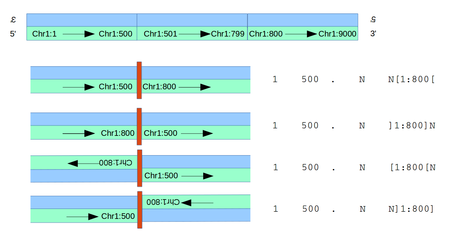
To describe a structural variant, we need more than just two positions, one per breakend. The breakends aren’t just points; they can be thought of as half-intervals, (eg, the piece of Chromosome 1 leading up to position 500; or the piece of Chromsome 1 starting at and continuing from position 500), and we will need that directional information.
(In the VCF spec, from the diagrams it is pretty clear that these are closed intervals; eg, regardless of the direction of the half-interval, the interval includes position 500. It is not 100% clear to me that every caller that uses BND notation honours that convention, but since we’re using 300-bp windows, such off-by-one errors in location need not concern us here.).
Once that is established, there is one more piece of information which need to be established to define the adjacency between breakends A and B; it can be thought of in two equivalent ways. One is the relative orientation; is half-interval A joined after half-interval B, or before? The second is the (relative) strandedness. Are the two half-intervals joined in such a way that the same strands are joined, or are the strands reversed, as in an inversion?
In VCF BND notation, for consistency with other entries but perhaps somewhat confusingly, only the chromosome and position of the first breakpoint are listed, and then in the ALT field is encoded:
- The other chromosome and position of the other breakend (eg, 1:800 in the diagrams above)
- The orientation of the second breakend; whether this is the half-interval which starts at the given position and extends rightwards,
[1:800[, or extends from the left and ends at the position given,]1:800]. - Finally, the relative orientation of the first breakpoint and its direction is specified using the position of other bases relative to the second breakpoint.
- In the examples in the figure, ‘N’ is given in the REF field; the position of that N relative to the
]1:800]or[1:800[tells you whether the breakpoint involving 1:500 is joined before or after. - If after, it is the half-interval including that position and extending rightwards, other it is the breakpoint including that position extending to the left.
- That combined with the relative orientation of the second interval is enough to establish the adjacency.
- The
N, of course, could be a real base, if known; and the corresponding bases listed in the ALT field could be one or more different bases, as would be the case if a substitution occurred at or insertion occured between the two half-intervals being joined at the new adjacency.
- In the examples in the figure, ‘N’ is given in the REF field; the position of that N relative to the
Note that the adjacency can be described equally well from either side; that is, for the purposes of identifying the new adjacency we could just as easily list 1:800 first:
| 500 first | 800 first |
|---|---|
1 500 . N N[1:800[ |
1 800 . N ]1:500]N |
1 500 . N ]1:800]N |
1 800 . N N[1:500[ |
1 500 . N [1:800[N |
1 800 . N [1:500[N |
1 500 . N N]1:800] |
1 800 . N N]1:500] |
When flipping the order of the breakpoints, we either do nothing else (in the case of adjacencies with different relative strandedness/orientation) or also flip position and direction (in the case of adjacencies with the same relative orientation). Otherwise, we end up describing a different novel adjacency involving the same two positions.
Because we want to merge equivalent adjacencies, and some callers call an adjacency from both sides and others just from one, we normalize the order by always listing the lexicographically first breakpoint position first.
Symbolic Notation Translocations (<TRA>)
The other way given for describing a structural variant is with “symbolic notation”; listing meaningful tags like <INV> to describe an inversion, or <DUP> to describe a duplication, in the ALT field of a VCF record.
The most general of these is the translocation symbolic call, <TRA>, which isn’t covered in the VCF standard, which essentially works the same way as a BND-style call. However, since the ALT field is now occupied, we need some other way to put the information about the position of the second breakpoint, and the relative orientation of the two half-intervals.
The other position is listed in the INFO field, with the chromosome given in an entry called CHR2, and the position in an entry called END. That leaves the relative orientation with which they are joined.
Although again this doesn’t appear to be covered in the VCF specification, the convention is to use a “connection” field, CT, to indicate whether the 5’ or the 3’ end of the interval involving the first breakpoint position is connected to the 5’ or 3’ end of that involving the second. This gives the directions of both half-intervals and their connection, which is enough to define the adjacency.
We can then translate between BND notation and translocation calls:
| BND | <TRA> with CT INFO field |
|---|---|
1 500 . N N[1:800[ |
1 500 . N <TRA> ... CHR2=1;END=800;CT='3to5' |
1 500 . N ]1:800]N |
1 500 . N <TRA> ... CHR2=1;END=800;CT='5to3' |
1 500 . N [1:800[N |
1 500 . N <TRA> ... CHR2=1;END=800;CT='5to5' |
1 500 . N N]1:800] |
1 500 . N <TRA> ... CHR2=1;END=800;CT='3to3' |
Note again that the adjacencies can be described from either side. To flip these calls is fairly straightforward; the ends of the intervals (5’ or 3’) belong to their respective breakpoint positions, so flipping the breakpoints just means flipping the positions, and the first and second number in the CT record. So 3to3 and 5to5 remain the same, while 3to5 becomes 5to3 and vice versa.
Clearly, both
Higher-level Symbolic Calls (<DEL>, <INV>, <DUP>)
Higher-level calls have to be handled a little differently. Because some callers may call them using BND-style calls, or even <TRA> calls, they have to be decompose into the lowest common denominator - individual adjacencies.
In the figure below are simple examples of a deletion, an inversion, and a duplication.
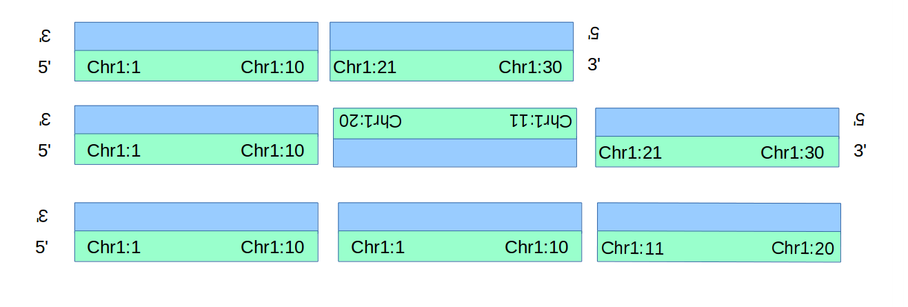
The deletion and duplication each generate only one novel adjacency (the 3to5 adjacency between Chr1:10 and Chr1:11 isn’t novel!), wheras the inversion generates 2.
Converting these into BND-style descriptions of the adjacencies follows below.
| Symbolic Call | As BND call(s) |
|---|---|
1 10 . N <DEL> ... END=20; |
1 10 . N N[1:21[ |
1 10 . N <INV> ... END=20; |
1 10 . N N]1:20] |
1 11 . N [1:21[N |
|
1 1 . N <DUP> ... END=10; |
1 1 . N ]1:10]N |
Breaking up calls like inversions into multiple calls proved important for understanding the comparison of results; we found several cases where some callers called an inversion, whereas others only identified one-half of the event.
Complications
While the above points cover most of the cases, the rather loose standards in this area cause a number of small bookkeeping headaches.
While callers often specify CT info fields for symbolic calls, they typically aren’t necessary (and are sometimes inconsistent with the intent of the caller, so suggesting an inverted duplication where a simple duplication is meant, or turning a deletion into a strange translocation, so we strip them out rather than interpreting them.
Similarly, some callers make BND-like calls but use SVCLASS info fields to label the call as a higher-level symbolic call, sometimes then leaving out other information which must then be inferred from the SVCLASS; these then have to be interpreted partly as BND-style calls and partly as symbolic calls.
Implementation
We are consider structural variants to be equal for the purposes of merging if they represent a novel adjacency between two “equivalent” breakends. We do not distinguish between calls that (for instance) have insertions called at the new adjacency.
As with the simple variants, these variants are stored as a python dictionary-of-dictionaries. Each dictionary is a “locationdict”, taking as a key a (chromosome, position, direction/strand) pair, and querying a key will match any position within the windowsize of that location. The first key is the (lexicographically first) breakpoint location and direction/strand, and the second is the that of the second. The final value is a list of callers making the call, and their VCF records for comparison.
By including direction/strand information, we avoid the issue of merging two breakpoints with positions close but indicating opposite half-intervals. So for instance, in the inversion example above, ]1:20] and [1:21[ are clearly very close together in their starting locations; but they must not be merged, as they are entirely non-overlapping regions.
Conclusion
Identifying common SV calls between two different callers with different conventions for outputting VCF records isn’t a deep algorithmic problem, but lack of consistent documentation makes it more challenging than we had originally anticipated. We hope that this writeup helps others who are need to do something similar.