On Random vs. Streaming I/O Performance; Or Seek(), and You Shall Find – Eventually.

Last week, Titus Brown asked a question on twitter and github which spurred a lot of discussion – what was the best way to randomly read a subset of entries in a FASTQ file? He and others quickly mentioned the two basic approaches – randomly seeking around in the file, and streaming the file through and selecting at random – and there were discussions of the merits of each in both forums.

This workload is a great case study for looking some of the ins and outs of I/O performance in general, and the tradeoffs between streaming and random file access in particular. The results can be a little surprising, and the exact numbers will necessarily be file system dependant: but on hard drives (and even more so on most cluster file systems), seeks will perform surprisingly poorly compared to streaming reads (the “Reservoir” approach in the plot below):

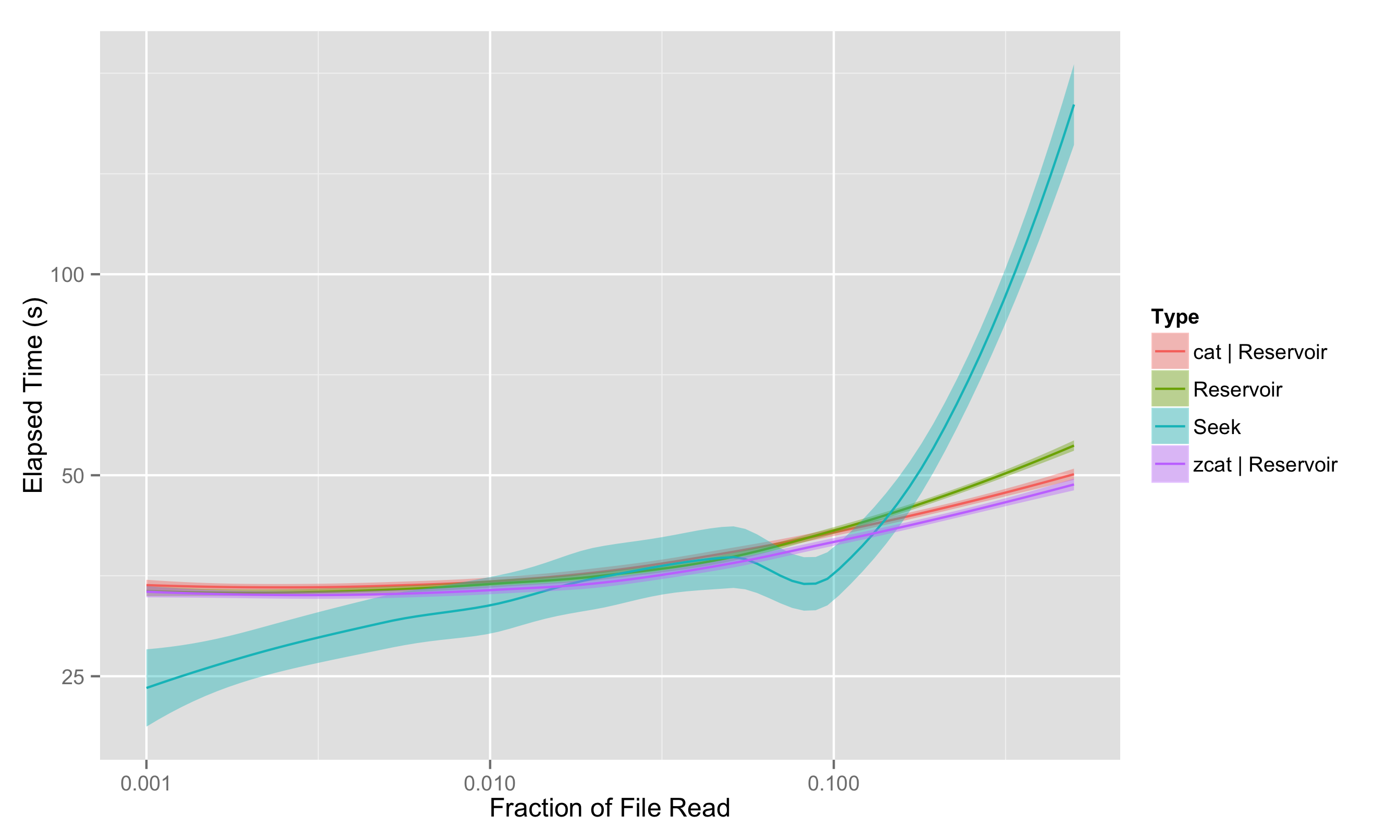
and here we’ll talk about why.

Anatomy of a File System

Unlike so many other pieces of software we have to deal with daily, the file system stack just works, and so we normally don’t have to spend much time thinking about what happens under the hood; but some level of familiarity with the moving parts in there and how they interact helps us better understand when we can and can’t get good performance out of that machine.

IOPS vs Bandwidth

A hard drive is a physical machine with moving parts, and the file system software stack is built around this (even in situations where this might not make sense any more, like with SSDs - about which more later). Several metal platters are spinning at speeds from 7,200 to 15,000 revolutions per minute (a dizzying 120-500 revolutions per second), and to start any particular read or write operation requires the appropriate sector of the disk being under the read heads; an event that won’t happen, on average, until 1 to 4 milliseconds from now.

Both the drive controller hardware and the operating system work hard to maximize the efficiency of this physical system, re-arranging pending reads and writes in the queue to ensure that requests are processed as quickly as possible; this allows one read request to “jump the queue” if the sector it needs to read from is just about to arrive, rather than having it wait in line, possibly for more than one disk rotation. While this can greatly help the throughput of a large number of unrelated operations, it can’t do much to speed a single threaded program’s stream of reads or writes.

This means that, for physical media, there is a limit to the number of (say) read I/O Operations Per Second (IOPS) that can be performed; the bottleneck could be at the filesystem level, or the disk controller, but it is normally at the level of the individual hard drive, where the least can be done about it. As a result, even for quite good, new, hard drives, a typical performance might be say 250 IOPS.

On the other hand, once the sector is under the read head, a lot of data can be pulled in at once. New hard disks typically have block sizes of 4KB, and all of that data can be slurped in essentially instantly. A good hard disk and controller can easily provide sequential read rates (or bandwidth) of over 100MB/s.

Prefetching and Caching, or: Why is Bandwidth so good?

You, astute reader, will have noticed that the numbers in that sentence above don’t even come close to working out. 250 IOP/s times 4KB is something like 1 MB/s, not 100MB/s. Where does that extra factor of 100 come from?

Much as the operating system and disk controller both work to schedule reads and writes so that they are collectively completed as quickly as possible, the entire input/output stack on modern operating systems is built to make sure that it speeds up I/O whenever possible – and it is extremely successful at doing this, when the I/O behaves predictably. Predictable, here, means that there is a large degree of locality of reference in the access; either temporal locality (if you’ve accessed a piece of data recently, you’re likely to access it again), or spatial (if you’ve accessed a piece of data, you’re likely to access a nearby piece soon).

Temporal locality is handled through caching; data that is read in is kept handy in case it’s needed again. There may be block caches on the disk drive or disk controller itself; within the Linux kernel there is a unified cache which caches both low-level blocks and high level pages worth of data (the memory-mapped file interface ties directly into this). Directory information is cached there, too; you may have noticed that in doing an ls -l in a directory with a lot of files, the first is much slower than any followups.

In user space, I/O libraries often do their own caching, as well. C’s stdlib, for instance, will cache substantial amounts of recently used data; and so, by extension, will everything built upon it (iostreams in C++, or lines of data seen by Python). The various players are shown below in this diagram from IBM’s DeveloperWorks:

None of this caching directly helps us in our immediate problem, since we’re not intending to re-read a sequence again and again; we are picking a number of random entries to read. However, the entire mechanism used for caching recently used data can also be used for presenting data that the operating system and libraries thinks is going to be used soon. This is where the second locality comes in; spatial locality.

The Operating System and libraries make the reasonable assumption that if you are reading one block in a file, there’s an excellent chance that you’ll be reading the next block shortly afterwards. Since this is such a common scenario, and in fact one of the few workloads that can easily be predicted, the file system (at all levels) supports quite agressive prefetching, or read ahead. This basic idea – since reading is slow, try to read the next few things ahead of time, too – is so widely useful that it is used not just for data on disk, but for data in RAM, links by web browsers, etc.

To support this, the lowest levels of the file system (block device drivers, and even the disk and controller hardware) try to lay out sequential data on disk in such a way that when one block is read, the next block is immediately ready to be read, so that only one seek, one IOP, is necessary to begin the read, and then following reads happen more or less “for free”. The higher levels of the stack take advantage of this by explicitly requesting one or many pages worth of data whenever a read occurs, and presents that data in the cache as if it had already been used. Then this data can be accessed by user software without expensive I/O operations.

The effectiveness of this can be seen not only in the factor of 100 difference in streaming reads (100MB/s vs 4KB x 250 IOP/s), but also in how performance suffers when this isn’t possible. On a hard drive that is nearly full, a new file being written doesn’t have the luxury of being written out in nice contiguous chunks that can be read in as a stream. The disk is said to be fragmented, and defragmentation can often improve performance.

In summary, then, prefetching and caching performed by the disk, controller, operating system, and libraries can speed large streaming reads on hard disks by a factor of 100 over random seek-and-read patterns, to the extent that, on a typical hard drive, 100-400KB can be read in the time that it takes to perform a single seek. On these same hard drives, then, you might expect streaming through a single 1000MB file to take roughly as long (~10s) as 2,500-4,000 seeks. We’ll see later that considering other types of file systems - single SSDs, or clustered file systems - can change where that crossover point between number of seeks versus size of streaming read will occur, but the basic tradeoff remains.

The Random FASTA Entry Problem

To illustrate the performance of both a seeking and sequential streaming method, let’s consider a slightly simpler problem than posed. To avoid the complications with FASTQ, let’s consider a sizeable FASTA file (we take est.fa from HG19, slightly truncated for the purposes of some of our later tests). The final file is about 8,000,000 lines of text, containing some 6,444,875 records. We consider both compressed and uncompressed versions of the file.

We’ll randomly sample \(k\) records from this file – 0.1%, 0.2%, 0.5%, 1%, 2%, 5%, 10%, 20%, and 50% of the total number of records \(N\) – run for several different trials, and done a few different ways. We’ll consider a seeking solution and a sequential reading solution.

The code we’ll discuss below, and scripts to reproduce the results, can be found on GitHub. The code is in Python, for clarity.

A Seeking Solution

Coding up a solution to randomly sample the file by seeking to random locations is relatively straightforward. We generate a random set of offsets into the file, given the file’s size; then seek to each of these locations in order, find and read the next record, and continue.

def randomSeek(infile, size, nrecords):
    infile.seek(0, os.SEEK_SET)

    totrecords = 0
    recordsdict = {}
    while totrecords < nrecords:
        # generate the random locations
        locations = []
        for i in range(nrecords-totrecords):
            locations.append(int(random.uniform(0,size)))
        locations.sort()

	# read the records immediately following these locations
        reader = simplefasta.FastaReader(infile)
        for location in locations:
            infile.seek(location,os.SEEK_SET)
            reader.skipAhead()
            record = reader.readNext()
            recordsdict[record[0]] = record[1]
        totrecords = len(recordsdict)
        
    # return a list of records
    records = []
    for k,v in recordsdict.items():
        records.append((k,v))
    return records

There are a few things to note about this approach:

• I’ve sorted the random locations to improve our chances of reading nearby locations sequentially, letting the operating system help us when it can.
• The file size must be known before generating the locations. This means we must have access to the whole file; we can’t just pipe a file through this method
• Some compression methods become difficult to deal with; one can’t just move to a random location in a gzipped file, for instance, and start reading. Other compression methods - bgzip, for instance, make things a little easier but still tricky.
• The method is not completely uniformly random if the records are of unequal length; we are more likely to land in the middle of a large record than a small one, so this method is biased in favour of records following a large one.
• Because we are randomly selecting locations, we may end up choosing the same record more than once; this gets more likely as the fraction of records we are reading increases. In this case, we go back and randomly sample records to make up the difference. There’s no way to know in general if two locations indicate the same record without reading the file at those locations.

A Streaming Solution - Reservoir Sampling

A solution to the \(k\)-random-sampling problem which makes use of streaming input is the Reservoir Sampling approach. This elegant method not only takes advantage of streaming support in the file system, but doesn’t require knowledge of the file size ahead of time; it is a so-called ‘online’ method.

The basic idea is that, for every \(i\)th item seen, it is selected with a probability of \(k/i\). Because there’s a \(1/(i+1)\) chance of it being bumped by the next item, then the probability of the \(i\)th item being selected by the end of round \(i+1\) is

and so on until by the time all \(N\) items are read, each item has a \(k/N\) chance of being selected.

Our simple implementation follows; we select the first \(k\) items to fill the reservoir, and then randomly select through the rest of the file.

def reservoir(infile, nrecords):
    reader = simplefasta.FastaReader(infile)
    results = [0]*nrecords
    for i in range(nrecords):
        results[i] = reader.readNext()

    countsSoFar = nrecords
    while not reader.eof():
        loc = random.randint(0,countsSoFar-1)
        if loc < nrecords:
            record = reader.readNext()
            if record:
                results[loc] = record
        else:
            reader.skipAhead(True)
        countsSoFar += 1
    return results

Note that this method does uniformly select records, and can work in pipes or through compressed files equally well as it passes sequentially through the entire file.

Timing Results: Workstation Hard Drive

I ran these benchmarks on my desktop workstation, with a mechanical hard drive. As a quick benchmark for streaming, simply counting the number of lines of the uncompressed (a shade under 4GB) file takes about 25 seconds on this system, which gives us a sense of the best possible streaming time for the file; this is about 160MB/s, a reasonable result (and in fact slightly higher than I would have expected). Similarly, if we expected an IOPS rate of about 400, then we’d expect to see 0.1% selection to take about 6445/400 ~ 16s.

The file handling and parsing will be significantly slower in python than it would be in C++, which disadvantages the streaming approach (which must process many more records than the seeking approach) somewhat, but our results should be instructive regardless.

The primary results are shown in this plot, which we have already seen (note that both x and y scales are logarithmic):

Some basic takeaways:

• The reservoir approach, which always has to pass through the entire file, is much less variable in time than the seeking approach.
• For sampling less than 0.75% of the file, seeking is clearly and reliably faster; for greater sampling fraction, seeking may or may not be faster
• At very large fractions, the seeking time blows up as the chance of “collisions” - selecting the same entry multiple times - greatly increases, meaning you have to go back and resample. But no one would really suggest this approach for sampling more than 10% of the file anyway.
• Reservoir sampling works roughly equally well if it is operating directly on the file or having it piped through; and it actually can be somewhat faster for a gzipped file with zcat, since less data actually has to be pulled from the disk.

We also tried the same test on gzipped files directly, since Python’s gzipped file access has a seek operation you can in principle use; but this isn’t really a fair test, as you can’t properly seek through a gzipped file, you have to decompress along the way. That means the “seeking” approach is really just a streaming approach implemented much less efficiently, and we see that quite clearly:

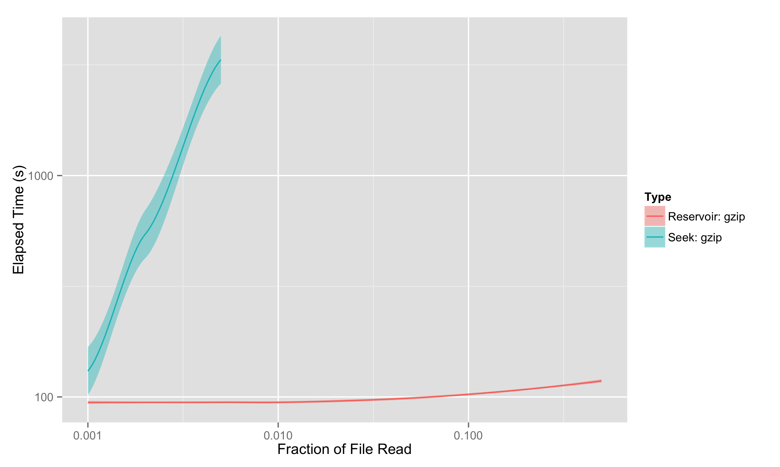
It was because the file was truncated that we could use gzip with seek-based sampling here at all; seek-sampling requires knowing the filesize, and the total (uncompressed) file size isn’t available with a gzipped file unless the uncompressed size is less than 4GB.

Sidebar - Benchmark warning: Clear that cache!

Note that for benchmarking I/O, even for moderately large files like this one (~1+GB compressed, 4GB uncompressed), a significant amount of the file will remain in various levels of OS cache, so it is absolutely essential to clear or avoid the cache in subsequent runs or else your timing results will be completely wrong.

On linux, as root, you can completely clear caches with the following:

$ sync
$ echo 3 > /proc/sys/vm/drop_caches

but this is rather overkill, and requires root. Easier, but requiring more disk space (and a file system which is not too smart/aggressive about deduplication!) is to cycle between multiple copies of the same file. The getdata script makes 5 copies each of the compressed and uncompressed est.trunc.fa file to cycle through, which may or may not be enough.

Other File Stores: Cluster File Systems

Of course, single spinning disk performance isn’t all that a bioinformatician cares about. Two other types of file systems play a large role; file systems on shared clusters, and individual SSDs.

On a cluster file system, data is stored on a large array of spinning disks. This has performance advantages, and disadvantages.

On the plus side, file systems like Lustre will often stripe large files across several disks and even servers, so that streaming reads can be served from many pieces of hardware at once – potentially offering many multiples of 100MB/s of streaming bandwidth. Similarly, the data file being striped across multiple disks means that many multiples of the IOPS are in principle available.

In practice, because so many parts (servers, disks) need to be coordinated to perform operations, there is often an additional latency to file system operations; this tends to come through as modestly fewer effective IOPS than one would expect. This means that the IOPS, while still potentially much higher than a local disk, are proportionally less increased than the bandwidth, tilting the balance in favour of streaming over seeking.

On the other hand, having a network-attached file system introduces another potential bottleneck; a slow or congested network may mean that the peak bandwidth available for streaming reads at the reader may be decreased, pushing the balance back towards seeking.

Other File Stores: SSDs

SSDs – which are ubiquitous in laptops and increasingly common on workstations – change things quite a bit. These solid state devices have no moving parts, meaning that there is no delay waiting for media to move to the right location. As a result, IOPS on these devices can be significantly higher. Indeed, traditional disk controllers and drivers become the bottleneck; a consumer-grade device plugged in as a disk will still be limited to 500MB/s and say 20k IOPS, while specialized devices that look more directly like external memory can achieve much higher speeds. (For those who want to know more about SSDs, Lee Hutchinson has an epic and accessible discussion of how SSDs work on Ars Technica; the article is from 2012 but very little fundamental has changed in the intervening three years).

At those rates, both streaming and seeking workflows see a performance boost, but the increase is much higher for IOPS. Rather than streaming a 1000MB file taking roughly as long as 2,500-4,000 seeks, it is now more like 40,000 seeks. That’s still finite, and each seek still takes roughly as much time as reading 25KB of data; but that factor of ten difference in relative rates will change the balance between whether streaming or seeking is most efficient for any given problem.

Running this same test on my laptop gives results as shown below:

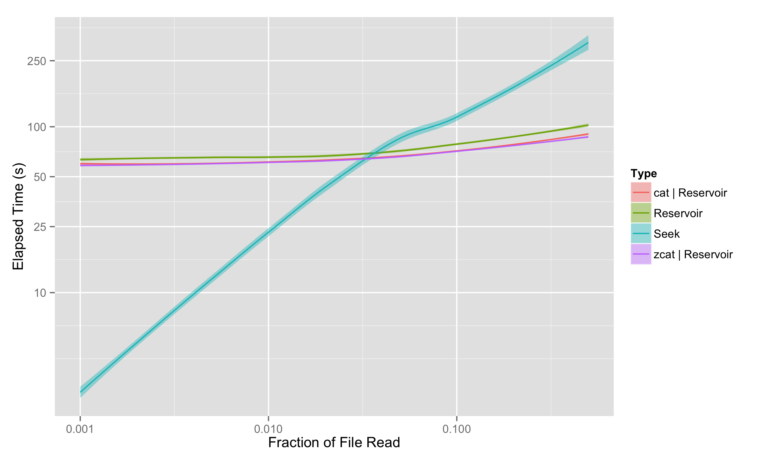
We see that the laptop-grade hardware limits the performance of the streaming read; bandwidths (and thus the performance of the reservoir sampling) are down by about a factor of 2. On the other hand, we seem to have gained over a factor of 10 in IOPS, with approximately 3000 effective random reading IOPS. As a result, the seeking for a 0.1% sampling fraction takes a lightning-fast 2.5 seconds.

However, it’s worth noticing that, even with the decrease in bandwidth and startling increase in IOPS, the crossover point between where streaming wins over seeking has only shifted from 0.75% to 3%; beyond that, streaming is clearly the winner.

How to further improve seeking results

Hardware: SSDs

Mechanical hard drives will always be at a significant disadvantage for random-access workloads compared to SSDs. While SSDs are significantly more expensive than mechanical HDs for the same capacity, the increase in performance for these workloads (and their lower power draw for laptops) may make them a worthwhile investment for use cases where seeky access can’t be avoided.

Software: multithreading

It’s also possible to improve the performance of the seeky workload through software. As mentioned before, the file system OS layer and physical layer are highly concurrent, juggling many requests at once and shuffling the order of requests behind the scenes to maximize throughput. For a highly seeky workflow like this, it’s often possible to make use of this concurrency by launching multiple threads, each sending their read request at the same time, and waiting until completion before launching the next. This greatly increases the chance of finding a read request which can be performed quickly, making fuller use of the disk subsystem. This significantly increases the complexity of the user software, however, and I won’t attempt it for the purposes of this post.

Software: turning off OS caching

A smaller possible gain could be realized, for small sample fractions, by hinting to the operating system not to provide expensive caching that will not be used by the seek-heavy access pattern. This can be done by opening the file with O_DIRECT, or using posix_fadvise which allows a more flexible method for hinting to the operating system not to bother prefetching or caching, respectively, by passing POSIX_FADV_RANDOM and POSIX_FADV_NOREUSE. However, this is likely only helpful for very small sample fractions, where seeking is already doing pretty well; for moderate sample fractions, the prefetching can actually help (e.g., that downward trend in time taken at around 10%) so I did not include this in the benchmark.

How to further improve sequential results

Hardware: SSDs

Workstation-class SSDs, with appropriate controllers, also offer a significant increase in streaming bandwidth over their mechanical counterparts, even if the increase is proportionally less than that in IOPS. 4-5x increases are not uncommon, and those would benefit the reservoir method here.

Software: Faster parsing

While Python is excellent for many purposes, there is no question but that it is slower than compiled languages like C++. FASTA parsing is quite simple, and for very small sampling fractions, there is no good reason that the resevoir solution should be a factor of two or more slower than running wc -l. This hurts the reservoir sampling more than the streaming, as the resevoir approach (which parses records which then get bumped later) must parse ~17 times more records in this test than the seeking method.

Software: turning off OS caching

While prefetching is essential for the streaming performance we have seen, there may be some modest benefit to turning off caching of the data we read in; after all, even with the reservoir sampling, we are still only processing each record at most once. Again, we could use posix_fadvise, this time with only POSIX_FADV_NOREUSE. I again expect this to be a relatively small effect, and so it is not tested here.

Conclusion: I/O is Complicated, But Streaming is Pretty Fast

This post only scratches the surface of I/O performance considerations. While we’ve thought a little bit about seeking vs sequential reading IOPS and bandwidth, even just streaming writes has different considerations (on the one hand, you can write anywhere that’s free, as opposed to needing to read specific bytes; on the other hand, there’s nothing like ‘prefetching’ for reads). More complex operations – and especially metadata-heavy operations, like creating, deleting, or even just appending to files – involve even more moving parts.

And even for seeking vs streaming reads, while the trends we’ve discussed here are widely applicable, different systems – underlying hardware (disk vs ssd) or how the file system is accessed (network-attached vs local) can greatly change the underlying numbers, which change the tradeoffs between seeking and streaming, possibly enough to make the conclusions different for any particular use case. We are empiricists, and the best way to find out which approach works best for your problem is to measure on the system that you use – fully aware that anyone else who uses your software might do so on different systems or for different-sized problems.

But a lot of software and hardware infrastructure is tuned to make streaming reads from filesystems as fast as possible, and it’s always worth testing to see if streaming through the data really isn’t fast enough.