Approximate Mapping of Nanopore Squiggle Data with Spatial Indexing
Nanopore data
Here at the Simpsonlab we work with signal-level data from nanopore sequencers, particularly those from ONT like the MinION. Signal-level data looks something like this:
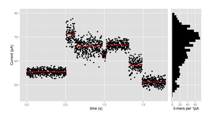
where the data comes in as a stream of events (the red lines) with means, standard deviations, and durations, with each black point being an individual signal reading. We use the signal-level data partly for accuracy - because converting each red line and dozens of black points into one of four letters invariably loses lots of information - and partly because those basecalls might not be available in, say, the field, where the portability of the nanopore sequencers really shines.
This data has to be interpreted in terms of a particular model of the interaction of the pore and the strand of DNA; such a pore model gives, amongst other things, an expected signal mean and standard deviation for currents through the pore when a given \(k\)mer is in the pore (for the MinION devices, pore models typically use \(k\)=5 or 6). So a pore model might be, for \(k\)=5, a table with 1024 entries that looks something like this:
| kmer | mean | std dev |
|---|---|---|
| AAAAA | 70.24 | ± 0.95 pA |
| AAAAC | 66.13 | ± 0.75 pA |
| AAAAG | 70.23 | ± 0.76 pA |
| AAAAT | 69.25 | ± 0.68 pA |
| … | … | … |
and using such a pore model it’s fairly straightforward to go from a sequence to an expected set of signal levels from the sequencer: so, say, for the 10-base sequence AAAAACGTCC and the above 5-mer pore model we’d expect 6 events (10-5+1) that look like:
| event | kmer | mean | range (1\(\sigma\)) |
|---|---|---|---|
| e1 | AAAAA | 70.2 pA | 69.3 - 71.2 pA |
| e2 | AAAAC | 66.1 pA | 65.4 - 66.9 pA |
| e3 | AAACG | 62.8 pA | 62.0 - 63.6 pA |
| e4 | AACGT | 67.6 pA | 66.3 - 68.9 pA |
| e5 | ACGTC | 56.6 pA | 54.5 - 58.7 pA |
| e6 | CGTCC | 49.9 pA | 49.1 - 50.7 pA |
Using those models, plus HMMs and a tonne of math, Jared’s nanopolish tool has had enormous success improving the quality of nanopore reads and assemblies of nanopore data. As one can see from the ‘range’ column above, and from the histogram on the side of the first plot, which shows the numbers of kmers which fall into 1pA bins in the pore model, this isn’t necessarily particularly easy. There are over 70 kmers which are expected to have means in the range 69.5pA - 70.5pA; that plus the wide standard deviations means that there is enormous ambiguity going back from signal levels to sequence.
Mapping
This ambiguity introduces complication into another part of the bioinformatics pipeline - mapping. While several mappers (BWA MEM, LAST) work quite well with basecalled ONT data, and one mapper1 has been written specifically for basecalled ONT data, mapping signal-level data directly is a little tougher. It is one thing for a seed sequence in the read to occur in multiple locations in the reference index; it is another thing for a sequence of floating-point currents to plausibly represent one of hundreds of seed sequences.
On the other hand, a flurry of recent important papers and software2
3 4 5, the first of which are discussed in some informative
blog
posts,
have demonstrated the usefulness of approximate read mapping. In
our case, mapping to an approximate region of a reference would
allow exact but computationally expensive methods like nanopolish
eventalign to produce precise alignments, or simple assignment may
be all that is necessary for other applications.
So an output approximate mapping would be valuable, but the issues remains of how to disambiguate the signal level values.
Spatial Indexing
Importantly, while any individual event is very difficult to assign with precision, sequences of events are less ambiguous, as any given event is followed, with high probability, by one of only four other events. Thus, by examining tuples of events, one can greatly increase specificity.
And there are well-developed sets of techniques for looking up lists of \(d\) floating point values to look for candidate matches: spatial indexes, where each query or match is considered as a point in \(d\)-dimensional space, and the goal is to return either some number of nearest points (k-Nearest-Neighbours, or kNN queries), or all matches within some, typically euclidean, distance.
To see how this would work, consider indexing the sequence above, AAAAACGTCC, in a spatial index with \(d=2\). There are a total of 6 events, so we’d have 5 points (6-2+1), each points in 2-dimensional space; 4 are plotted below (the other falls out of the range of the plot)
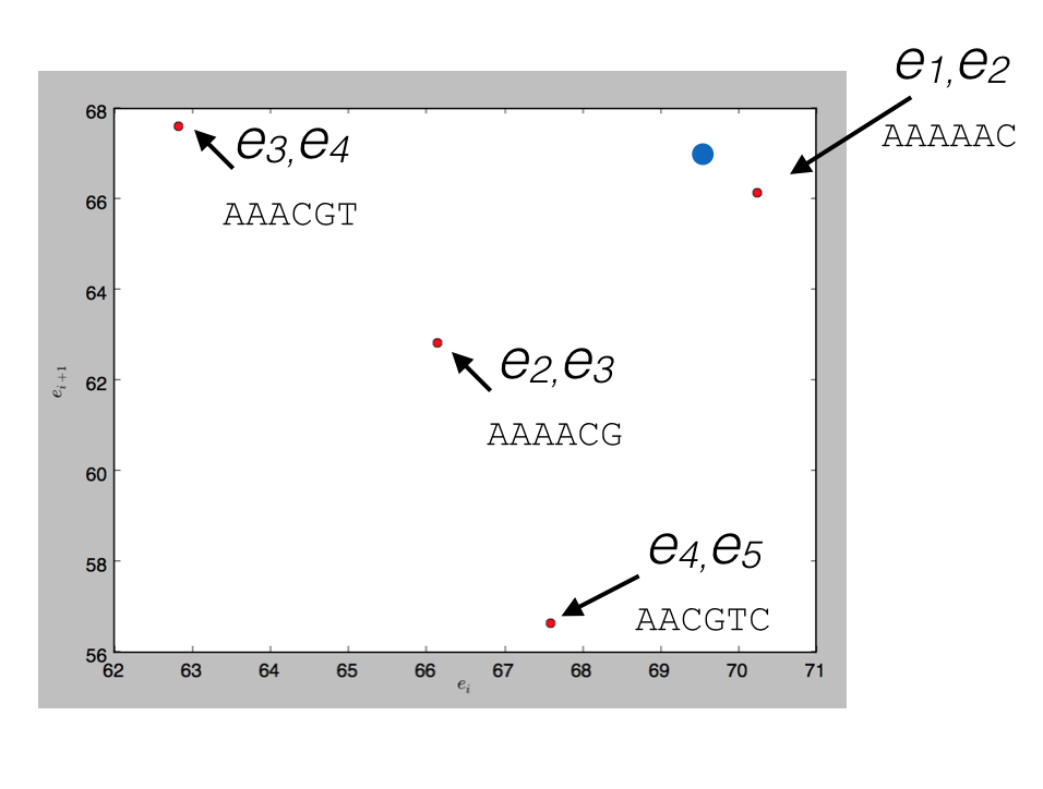
and a query for \(d\) read events that could be matched by (69.5, 67), the blue point, would return the nearest match (70.2, 66.1) corresponding to the \(k+d-1\)-mer AAAAAC.
So to map event data, one can:
- Generate an index:
- Generate all overlapping tuples of \(d\) kmers from a reference
- Using a pore model, convert those into points in \(d\)-space
- Create a spatial index of those points,
- For every read:
- Take every overlapping set of \(d\) events
- Look it up in a spatial index
- Find a most likely starting point for the read in the reference, with a quality score.
Note that one has to explicitly index both the forward and reverse strands of the reference, since you don’t a priori know what the “reverse complement” of 65.5 pA is. One also has to generate multiple indices; for 2D ONT reads, there is a pore model for the template strand of a read, and typically two possible models to choose from for the complement strand of a read, so one needs three indexes in total to query.
What dimension to choose?
To test this approach, you have to choose a \(d\) to use. On the one hand, you would like to choose as large a dimension as you can; the larger \(k+d-1\) is, the more unique each seed is and the fewer places it will occur in any reference sequence.
On the other hand, two quite different constraints put a strong upper limit on the dimensions that will be useful:
- The curse of dimensionality - in high spatial dimensions, nearest-neighbour searching is extremely inefficient, because distance loses its discriminative power. (Most things are roughly equally far from each other in 100-dimensional space; there are a lot of routes you can take!) As a practical matter, for most spatial index implementations, for \(d > 15-20\) or so you might as well just do a linear search over all possible items;
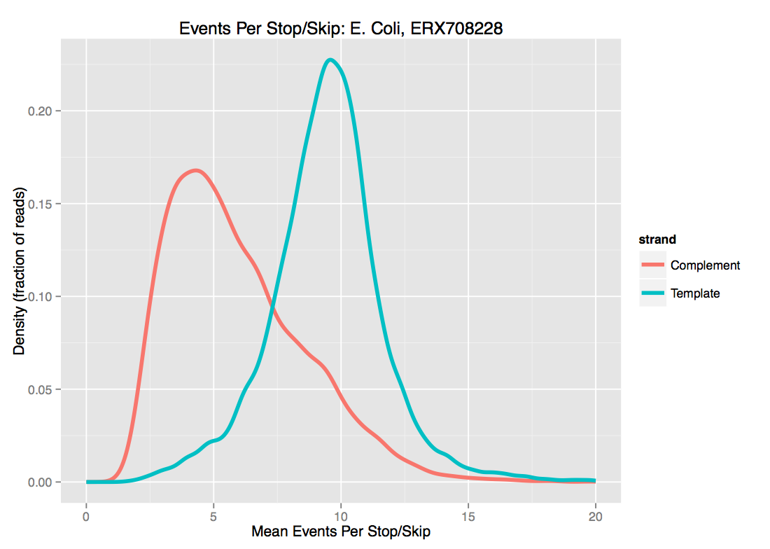
- Current approaches to segmentation mean that ONT data has very frequent ‘stops’ and ‘skips’ - that is, events are spuriously either inserted or deleted from the data. Exactly as with noisy basecalled sequences, this strongly limits the length of sequence that can be usefully used as seeds. As we see below for one set of E. coli data, there is probably not much point in using \(d \ge 10\) even for template-strand data, as the median “dmer” will have an insertion/deletion in it.
For these two reasons, we’ve been playing with \(d \approx 8\). I’ll note that while increasing \(d\) is the most obvious knob to turn to increase specificity of the match, higher \(k\) helps as well.
Normalizing the signal levels
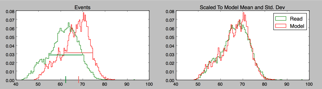
One issue we haven’t mentioned is that the raw nanopore data needs calibration to be compared to the model; there is an additive shift and drift over time, and a multiplicative scale that has to be taken into account.
A very simple “methods of moments” calculation works surprisingly well for long-enough reads, certainly well enough to start an iterative process; for any given model one is trying to fit a read to, rescaling the mean and standard deviation of read events to model events gives a good starting point for calibration, and drift is initially ignored.
Proof of concept
A simple proof of concept of using spatial indexing to approximately map squiggle data can be found on github. It’s written in python, and has scipy, h5py, and matplotlib as dependencies. Note that as implemented, it is absurdly memory-hungry, and definitely requires a numpy and scipy built against a good BLAS implementation.
As a spatial index, it uses a version of a k-d tree (scipy.spatial.cKDTree), which is a very versatile and widely used (and so well-optimized) spatial index widely used in machine learning methods amongst others; different structures may have advantages for this application.
Running the index-and-map.sh script generates an index for the provided ecoli.fa reference - about 1 minute per pore model - and then maps the 10 reads provided of both older 5mer and newer 6mer MAP data. Mapping each read takes about 6 seconds per read per pore model; this involves lots of python list manipulations so could fairly straightforwardly be made much faster.
Doing the simplest thing possible for mapping works surprisingly well. Using the same sort of approach as the first steps of the Sovic et al. method1, we just:
- Use the default k-d tree parameters (which almost certainly isn’t right, particularly the distance measure)
- Consider overlapping bins of starting positions on the reference, of size ~10,000 events, a typical read size
- For each \(d\)-point in the read,
- Take the closest match to each \(d\)-point (or all within some distance)
- For each match, add a score to the bin corresponding to the implied starting position of the read on the reference; a higher score for a closer match
- Report the best match starting point
Let’s take a look at the initial output for the older SQK005 ecoli data and newer SQK006 data:
$ ./index-and-map.sh

5mer data:

Indexing : model models/5mer/template.model, dimension 8
python spatialindex.py --dimension 8 ecoli.fa models/5mer/template.model indices/ecoli-5mer-template

real	0m52.922s
user	0m49.756s
sys	0m1.196s
Mapping reads: starting with ecoli/005/LomanLabz_PC_Ecoli_K12_R7.3_2549_1_ch182_file148_strand.fast5
time python ./mapread.py --plot save --plotdir plots --closest    --maxdist 3.5  \
    --templateindex indices/ecoli-5mer-template.kdtidx
    ecoli/005/LomanLabz_PC_Ecoli_K12_R7.3_2549_1_ch182_file148_strand.fast5 ...  > template-005-.txt

real	1m9.776s
user	1m9.108s
sys	0m1.004s
Template Only Alignments
Read           Difference  BWA      KDTree   zscore
ch277_file143  819         3079177  3079996  17.164000
ch498_file171  1130        3793866  3794996  11.916000
ch222_file28   1765        2803231  2804996  11.152000
ch461_file9    1895        2195243  2193348  8.749000
ch182_file148  2559        2767555  2764996  17.120000
ch34_file53    4772        1128120  1123348  11.235000
ch401_file98   4981        2328329  2323348  6.160000
ch80_file64    5649        4369347  4374996  7.469000
ch395_file89   5828        2069168  2074996  9.517000
ch464_file15   7031        2195379  2188348  14.782000
Indexing : model models/5mer/complement.model, dimension 8
python spatialindex.py --dimension 8 ecoli.fa models/5mer/complement.model indices/ecoli-5mer-complement

real	0m52.124s
user	0m47.948s
sys	0m1.332s

Mapping reads: starting with ecoli/005/LomanLabz_PC_Ecoli_K12_R7.3_2549_1_ch182_file148_strand.fast5
time python ./mapread.py --plot save --plotdir plots --closest    --maxdist 3.5  \
    --templateindex indices/ecoli-5mer-template.kdtidx  \
    --complementindex indices/ecoli-5mer-complement.kdtidx \
    ecoli/005/LomanLabz_PC_Ecoli_K12_R7.3_2549_1_ch182_file148_strand.fast5 ...  \
    > template-complement-005-.txt

real	1m47.590s
user	1m46.228s
sys	0m1.712s

Template+Complement Alignements
Read           Difference  BWA      KDTree   zscore
ch401_file98   19          2328329  2328348  7.516000
ch277_file143  819         3079177  3079996  17.164000
ch498_file171  1130        3793866  3794996  11.916000
ch222_file28   1765        2803231  2804996  11.152000
ch461_file9    1895        2195243  2193348  10.378000
ch182_file148  2559        2767555  2764996  17.120000
ch34_file53    4772        1128120  1123348  11.235000
ch80_file64    5649        4369347  4374996  7.469000
ch395_file89   5828        2069168  2074996  9.517000
ch464_file15   7031        2195379  2188348  14.782000

6mer data:

Indexing : model models/6mer/template.model, dimension 8
python spatialindex.py --dimension 8 ecoli.fa models/6mer/template.model indices/ecoli-6mer-template

real	1m4.028s
user	0m57.924s
sys	0m1.872s

Mapping reads: starting with ecoli/006/LomanLabz_PC_Ecoli_K12_MG1655_20150924_MAP006_1_5005_1_ch102_file146_strand.fast5
time python ./mapread.py --plot save --plotdir plots --closest --maxdist 3.5 \
    --templateindex indices/ecoli-6mer-template.kdtidx \
    ecoli/006/LomanLabz_PC_Ecoli_K12_MG1655_20150924_MAP006_1_5005_1_ch102_file146_strand.fast5 ...  > template-006-.txt

real	1m46.643s
user	1m45.636s
sys	0m1.276s
Template Only Alignments
Read           Difference  BWA      KDTree   zscore
ch383_file65   844         89152    89996    20.490000
ch209_file0    1119        4564467  4563348  24.038000
ch485_file6    1739        400087   398348   23.698000
ch179_file92   3113        496461   493348   16.477000
ch102_file146  4965        1378313  1373348  25.003000
ch241_file2    5625        1578973  1573348  5.919000
ch339_file119  5710        829058   823348   22.348000
ch412_file79   5806        2194190  2199996  19.218000
ch228_file128  5933        3809063  3814996  17.926000
ch206_file36   11173       4373823  4384996  28.011000

Indexing : model models/6mer/complement_pop1.model, dimension 8
python spatialindex.py --dimension 8 ecoli.fa models/6mer/complement_pop1.model indices/ecoli-6mer-complement_pop1
python spatialindex.py --dimension 8 ecoli.fa models/6mer/complement_pop2.model indices/ecoli-6mer-complement_pop2
[..]

Mapping reads: starting with ecoli/006/LomanLabz_PC_Ecoli_K12_MG1655_20150924_MAP006_1_5005_1_ch102_file146_strand.fast5
time python ./mapread.py --plot save --plotdir plots --closest --maxdist 3.5  \
    --templateindex indices/ecoli-6mer-template.kdtidx  \
    --complementindex indices/ecoli-6mer-complement_pop1.kdtidx,indices/ecoli-6mer-complement_pop2.kdtidx \
    ecoli/006/LomanLabz_PC_Ecoli_K12_MG1655_20150924_MAP006_1_5005_1_ch102_file146_strand.fast5 ...  > template-complement-006-.txt

real	3m55.773s
user	3m31.032s
sys	0m4.364s

Template+Complement Alignements
Read           Difference  BWA      KDTree   zscore
ch383_file65   844         89152    89996    20.490000
ch209_file0    1119        4564467  4563348  24.038000
ch485_file6    1739        400087   398348   23.698000
ch179_file92   3113        496461   493348   16.477000
ch102_file146  4965        1378313  1373348  25.003000
ch339_file119  5710        829058   823348   22.348000
ch412_file79   5806        2194190  2199996  19.218000
ch228_file128  5933        3809063  3814996  17.926000
ch241_file2    9375        1578973  1588348  11.626000
ch206_file36   11173       4373823  4384996  28.011000
We see a couple of things here:
- Adding the complement strand does almost nothing for the accuracy, but requires substantially more memory and compute time, as multiple indices must be loaded and used up, and all candidate complement indices must be compared against each other. Because of this and the typically higher skip/stay rates for complement strands, we will use the template strand only for the rest of this post;
- Since we are simply assigning starting bins at this point, any assignments within the bin size are equally accurate; here, all of the reads were correctly assigned to the starting bin or the neighbouring one.
- The newer 6mer data gives slightly better results; part of this is likely because we are using the same \(d\), so a dmer for the k=6 data corresponds to seed longer by one
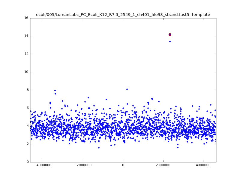
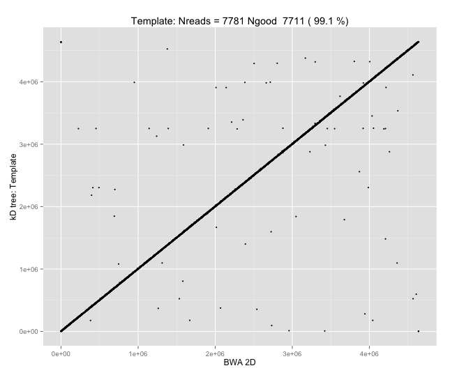
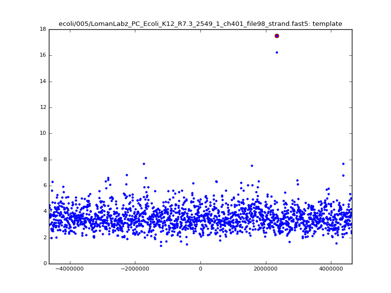
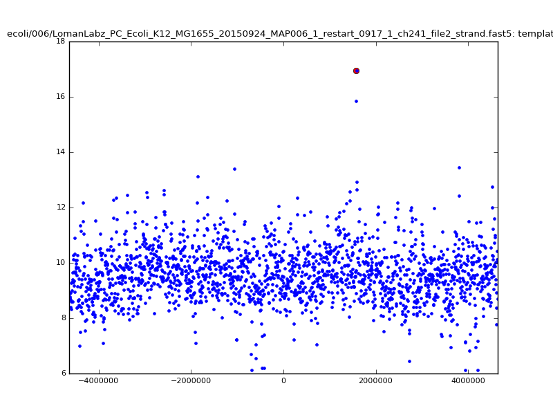
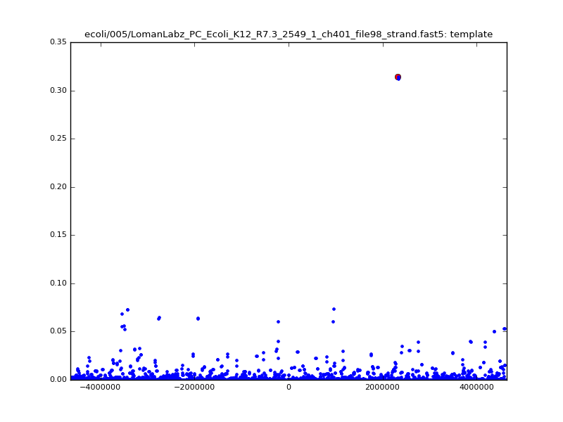
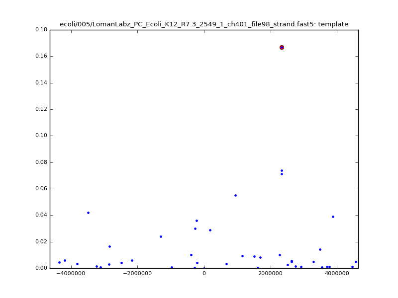
- The zscore here is a very crude measure of how much the assignment stands out over the background (but not necessarily how it compares to other candidate mappings); some of these very simple pseudo-mappings are relatively securely identified, and others less so. The sum-of-scores for the reads with the best and worst zscore results are plotted below; no prize for guessing which is which:
| 5mer | 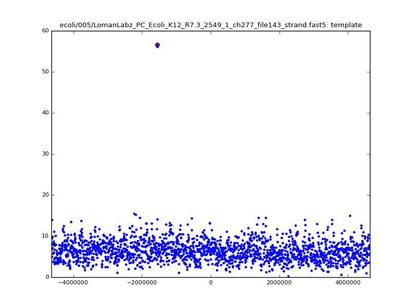 |
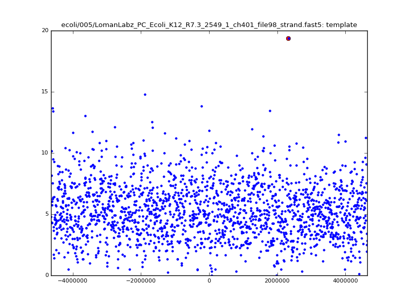 |
| 6mer | 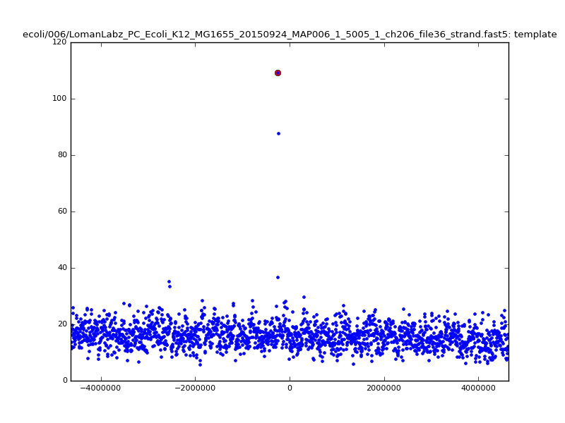 |
 |
Because many levels are clustered near ~60-70pA, many dmers are quite close to each other, and choosing simply the closest \(d\)-point is unlikely to give a robust result. Examining all possible matches in the spatial index within some given radius reduces the noise somewhat, at a modest increase in compute time:
$ ./index-and-map.sh noclosest templateonly
5mer data:
[...]
real 3m15.145s
user 3m5.840s
sys 0m2.972s
Template Only Alignments
Read Difference BWA KDTree zscore
ch401_file98 19 2328329 2328348 11.359000
ch277_file143 819 3079177 3079996 19.103000
ch498_file171 1130 3793866 3794996 15.353000
ch222_file28 1765 2803231 2804996 17.583000
ch182_file148 2559 2767555 2764996 18.579000
ch34_file53 4772 1128120 1123348 16.615000
ch80_file64 5649 4369347 4374996 10.181000
ch395_file89 5828 2069168 2074996 13.145000
ch461_file9 6895 2195243 2188348 10.431000
ch464_file15 7031 2195379 2188348 18.042000
6mer data:
[...]
real 9m29.562s
user 9m9.536s
sys 0m16.600s
Template Only Alignments
Read Difference BWA KDTree zscore
ch383_file65 844 89152 89996 21.777000
ch485_file6 1739 400087 398348 24.384000
ch179_file92 3113 496461 493348 19.718000
ch102_file146 4965 1378313 1373348 24.218000
ch241_file2 5625 1578973 1573348 7.311000
ch339_file119 5710 829058 823348 26.045000
ch228_file128 5933 3809063 3814996 20.042000
ch209_file0 6119 4564467 4558348 23.703000
ch412_file79 10806 2194190 2204996 21.677000
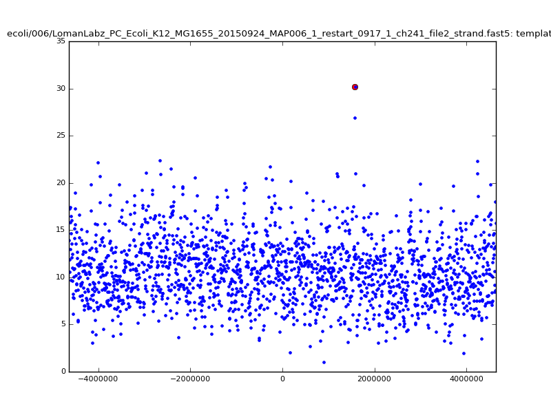
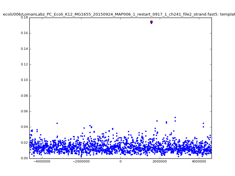
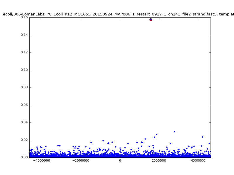
ch206_file36 11173 4373823 4384996 29.794000Note the increase in zscores; the same two reads are plotted:
| 5mer | 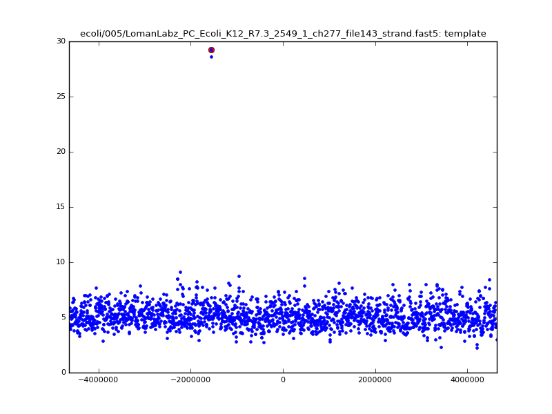 |
 |
| 6mer | 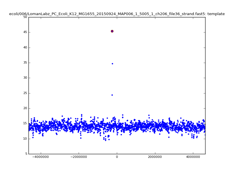 |
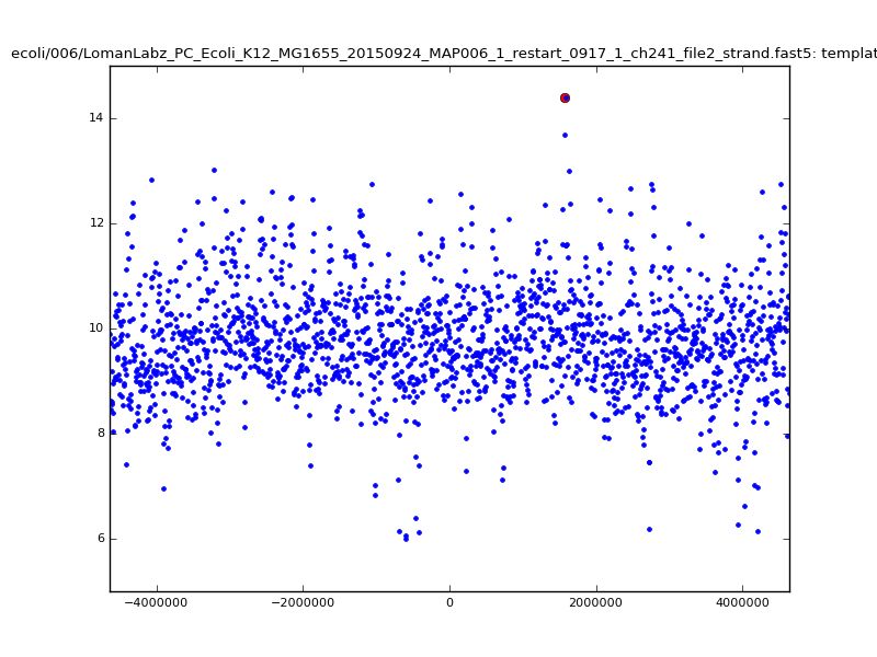 |
With a few other tweaks - keeping track of the top 10 candidates, and for each re-testing by recalibrating given the inferred mapping and rescoring - we can get about 95%-99% accuracy in mapping.
Of course, while 95-99% (Q13-Q20) mapping accuracy on E. coli is a cute outcome from such a simple approach, it isn’t nearly enough; with \(d=8\) and \(k=5\), wer’e working with seeds of size 12, which would typically be unique in the E. coli reference, but certainly wouldn’t be in the human genome, or for metagenomic applications.
EM Rescaling
One limiting factor is the approximate nature of the rescaling so far that is being performed; for reads that have been basecalled, the inferred shift values above can be off by several picoamps from the Metrichor values, which clearly causes both false negatives and false positives in the index lookup. This can be addressed by doing a more careful rescaling step, using EM iterations:
- For the E-step, provisionally assign probabilities of read events corresponding to model levels, based on the Gaussian distributions described in the model and a simple transition matrix between events;
- For the M-step, perform a weighted least squares regression to re-scale the read levels.
This gives answers that are quite good when compared with Metrichor, at the cost of substantially more computational effort (much greater than the spatial index lookup!), particularly for long reads and larger (k) where the number of model levels is larger:
$ ./index-and-map.sh noclosest templateonly rescale
5mer data:
[...]
real	7m1.866s
user	6m56.708s
sys	0m29.236s
Template Only Alignments
Read           Difference  BWA      KDTree   zscore
ch401_file98   19          2328329  2328348  14.975000
ch277_file143  819         3079177  3079996  22.516000
ch498_file171  1130        3793866  3794996  20.894000
ch222_file28   1765        2803231  2804996  19.569000
ch182_file148  2559        2767555  2764996  20.443000
ch34_file53    4772        1128120  1123348  17.401000
ch395_file89   5828        2069168  2074996  13.510000
ch461_file9    6895        2195243  2188348  11.165000
ch464_file15   7031        2195379  2188348  19.315000
ch80_file64    10649       4369347  4379996  15.109000

6mer data:
[...]
real	33m11.324s
user	31m55.172s
sys	2m0.836s
Template Only Alignments
Read           Difference  BWA      KDTree   zscore
ch383_file65   844         89152    89996    23.732000
ch179_file92   3113        496461   493348   20.845000
ch102_file146  4965        1378313  1373348  24.997000
ch241_file2    5625        1578973  1573348  10.574000
ch339_file119  5710        829058   823348   26.816000
ch228_file128  5933        3809063  3814996  21.397000
ch209_file0    6119        4564467  4558348  24.546000
ch485_file6    6739        400087   393348   24.790000
ch412_file79   10806       2194190  2204996  25.477000
ch206_file36   11173       4373823  4384996  30.164000
Note again the increase in zscores; replotting gives:
| 5mer | 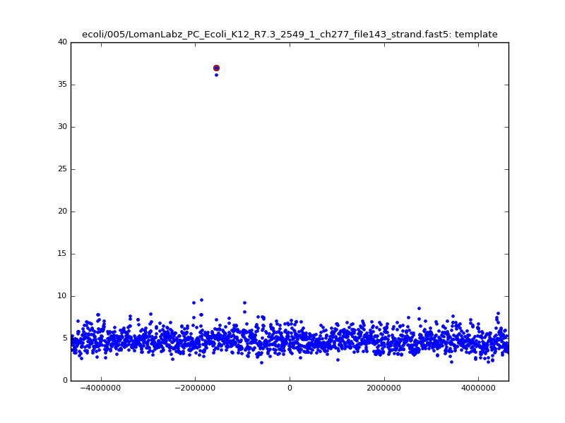 |
 |
| 6mer | 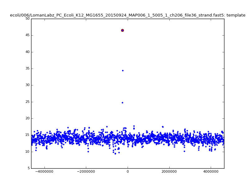 |
 |
Extending the seeds
So far we have in no way taken into account any of the locality information in the spatial index lookup results; that is, that a long series of hits close together, in the same order on the read and on the reference, is much stronger evidence for a good mapping than a haphazard series of hits in random order that happen to fall within the same bin of starting points.
Keeping with the do-the-simplest-thing approach that has worked so far, we can try to extend these “seed” matches by stitching them together into longer seeds; here we build 15-mers out of sets of 4 neighbouring 12-mers, allowing one skip or stay somewhere within them, using as a score for the result the minimum of the constituent scores, and dropping all hits that cannot be so extended. This has quite modest additional cost, and works quite well:
$ ./index-and-map.sh noclosest templateonly rescale extend
5mer data:

[...]
real	7m20.914s
user	7m19.228s
sys	0m23.620s
Template Only Alignments
Read           Difference  BWA      KDTree   zscore
ch498_file171  1130        3793866  3794996  28.762000
ch222_file28   1765        2803231  2804996  27.434000
ch461_file9    1895        2195243  2193348  29.089000
ch182_file148  2559        2767555  2764996  29.538000
ch34_file53    4772        1128120  1123348  28.837000
ch401_file98   4981        2328329  2323348  23.840000
ch277_file143  5819        3079177  3084996  29.832000
ch395_file89   5828        2069168  2074996  23.705000
ch464_file15   7031        2195379  2188348  28.941000
ch80_file64    10649       4369347  4379996  26.926000

6mer data:
[...]
real	33m57.863s
user	32m58.236s
sys	1m42.548s
Template Only Alignments
Read           Difference  BWA      KDTree   zscore
ch241_file2    625         1578973  1578348  25.137000
ch485_file6    1739        400087   398348   30.297000
ch339_file119  5710        829058   823348   31.856000
ch383_file65   5844        89152    94996    30.163000
ch228_file128  5933        3809063  3814996  29.294000
ch209_file0    6119        4564467  4558348  30.169000
ch179_file92   8113        496461   488348   28.732000
ch102_file146  9965        1378313  1368348  30.107000
ch412_file79   10806       2194190  2204996  30.377000
ch206_file36 11173 4373823 4384996 33.896000| 5mer |  |
 |
| 6mer | 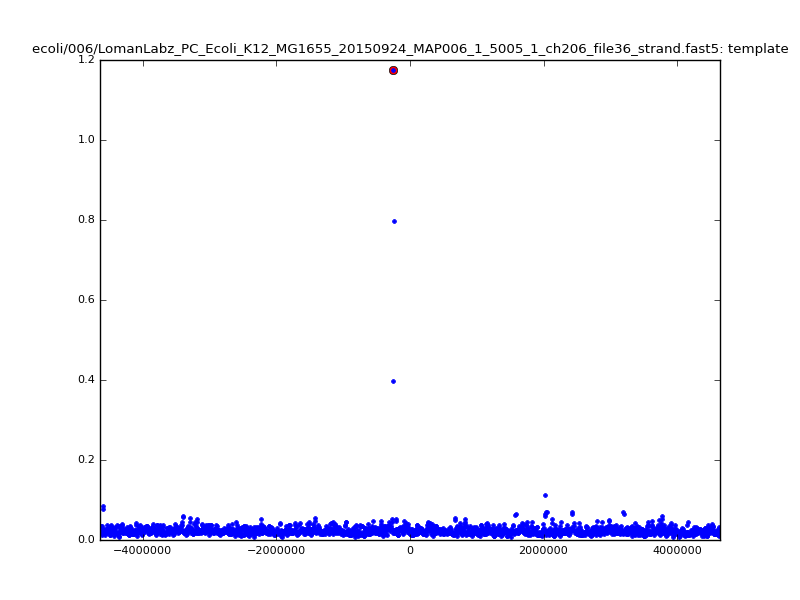 |
 |
Now that we seem to have much stronger and more specific results, we can investigate letting go of binning, and instead string these extended seeds into longest possible matches. Continuing to extend dmer-by-dmer is too challenging due to missing points (due to mis-calibration, too large noise in the dmer falling out of the maxdist window in the kdtree, or several skip/stays in a row), so following the ideas of graphmap1 and minimap5, we trace collinear seeds through the set of available seeds; rather than just taking longest increasing sequences in inferred start positions, however, we make a graph of seeds with edges connecting seeds that are monotonically increasing both in read location and reference location with ‘small enough’ jumps, and extract longest paths through this graph. The cost of this is smaller than the rescaling of the read.
Running this, the zscores now somewhat change meaning; only the extracted paths are scored, meaning that the scores are only amongst plausible mappings, not over all bins across the reference. Similarly, the differences in mapping locations are somewhat more meaningful - rather than being compared to bin centres, they are actually the differences between mapping locations.
We get:
5mer data:
[...]

real	6m54.776s
user	6m52.064s
sys	0m23.648s
Template Only Alignments
Read           Difference  BWA      KDTree   zscore
ch461_file9    10          2195243  2195253  7.105000
ch34_file53    343         1128120  1128463  12.449000
ch401_file98   363         2328329  2328692  5.320000
ch464_file15   2826        2195379  2192553  13.267000
ch498_file171  3192        3793866  3797058  7.688000
ch182_file148  5450        2767555  2773005  10.107000
ch222_file28   5681        2803231  2808912  8.166000
ch277_file143  6381        3079177  3085558  9.190000
ch395_file89   7191        2069168  2076359  7.685000
ch80_file64    15167       4369347  4384514  7.965000


6mer data:
[...]

real	43m37.651s
user	42m37.208s
sys	1m42.848s
Template Only Alignments
Read           Difference  BWA      KDTree   zscore
ch209_file0    14          4564467  4564453  31.724000
ch485_file6    14          400087   400073   24.063000
ch241_file2    203         1578973  1578770  26.676000
ch179_file92   723         496461   495738   39.626000
ch339_file119  774         829058   828284   45.636000
ch102_file146  1568        1378313  1376745  45.601000
ch383_file65   5890        89152    95042    27.902000
ch228_file128  8120        3809063  3817183  35.863000
ch412_file79   13833       2194190  2208023  48.444000
ch206_file36 15650 4373823 4389473 38.441000| 5mer | 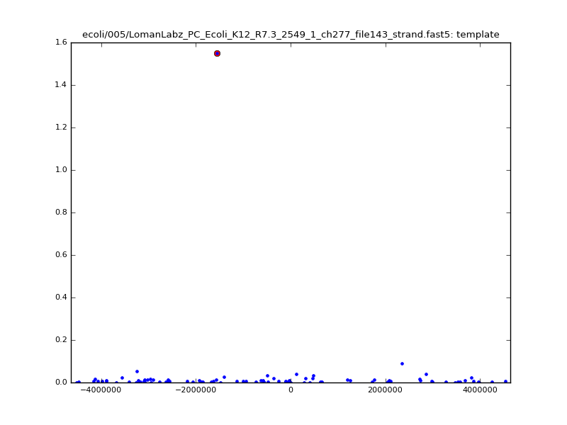 |
 |
| 6mer | 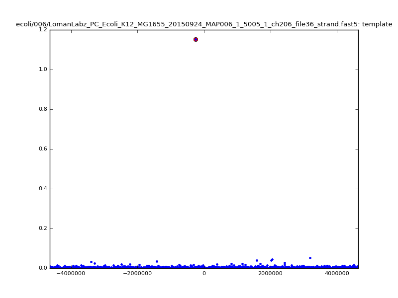 |
 |
The simple python testbed implementation of these ideas linked to above is very slow, single-threaded, absurdly memory hungry, and its treatment of scores for the mappings does not currently make much sense. In the new year we will address these issues in a proper C++ implementation, where (for instance) we will not have multiple copies of large, reference-sized data structures.
References
-
Fast and sensitive mapping of error-prone nanopore sequencing reads with GraphMap (2015) by Sovic, Sikic, Wilm, et al. ↩ ↩2 ↩3
-
Near-optimal RNA-Seq quantification (2015) by Bray, Pimentel, Melsted, and Pachter ↩
-
Salmon: Accurate, Versatile and Ultrafast Quantification from RNA-seq Data using Lightweight-Alignment (2015) by Patro, Duggal, and Kingsford ↩
-
Minimap and miniasm: fast mapping and denovo assembly for noisy long sequences, Heng Li ↩ ↩2